Application to NGC 7023

In this example, we consider a real cloud, NGC 7023, with observations already studied in Joblin et al. [2018].

Python Simulation preparation

Here are the classes that are necessary to sample from this distribution. The green classes indicate the already implemented classes, and the red classes indicate the classes to implement.

The class for inference based on

• real astrophysical data

• a neural network approximation

is already implemented: SimulationRealDataNN.

Therefore, the setup of the inversion is very simple, as one only needs to import and create an instance of this class.

ngc7023.py

import os

import numpy as np

from beetroots.simulations.astro import data_validation

from beetroots.simulations.astro.real_data.real_data_nn import SimulationRealDataNN

if __name__ == "__main__":
    yaml_file, path_data, path_models, path_outputs = SimulationRealDataNN.parse_args()

    # load ``.yaml`` file
    params = SimulationRealDataNN.load_params(path_data, yaml_file)

    SimulationRealDataNN.check_input_params_file(
        params,
        data_validation.schema,
    )

    # result of another estimation from the literature
    # note : G0 (front of cloud) = 1.2786 * radm / 2
    G0_joblin = 2.6e3
    radm_joblin = 2 * G0_joblin / 1.2786

    point_challenger = {
        "name": "Joblin et al., 2018",
        "value": np.array([[0.7, 1e8, radm_joblin, 1e1, 0.0]]),
    }

    # create simulation object and run its main method to launch the inversion
    simulation = SimulationRealDataNN(
        **params["simu_init"],
        path_data=path_data,
        path_outputs=path_outputs,
        path_models=path_models,
        forward_model_fixed_params=params["forward_model"]["fixed_params"],
    )

    simulation.main(
        params=params,
        path_data_cloud=path_data_cloud,
        point_challenger=point_challenger,
    )

YAML file

input_params_1p7_with_spatial_regu.yaml

simu_init:
    simu_name: "ngc7023"
    cloud_name: "ngc7023"
    max_workers: 10
    #
    params_names:
        kappa: $\kappa$
        P: $P_{th}$
        radm: $G_0$
        Avmax: $A_V^{tot}$
        angle: $\alpha$
    #
    list_lines_fit:
    - "co_v0_j11__v0_j10"
    - "co_v0_j12__v0_j11"
    - "co_v0_j13__v0_j12"
    - "co_v0_j15__v0_j14"
    - "co_v0_j16__v0_j15"
    - "co_v0_j17__v0_j16"
    - "co_v0_j18__v0_j17"
    - "co_v0_j19__v0_j18"
    #
    - "h2_v0_j2__v0_j0"
    - "h2_v0_j3__v0_j1"
    - "h2_v0_j4__v0_j2"
    - "h2_v0_j5__v0_j3"
    - "h2_v0_j6__v0_j4"
    - "h2_v0_j7__v0_j5"
    #
    - "chp_j1__j0"
    - "chp_j2__j1"
    - "chp_j3__j2"
#
to_run_optim_map: false
to_run_mcmc: true
#
filename_int: "Nebula_NGC_7023_Int.pkl"
filename_err: "Nebula_NGC_7023_Err.pkl"
#
forward_model:
    forward_model_name: "meudon_pdr_model_dense"
    force_use_cpu: false
    fixed_params: # must contain all the params in list_names of the SImulation object. Values are in linear scale.
        kappa: null
        P: null
        radm: null
        Avmax: null
        angle: 60.0
    is_log_scale_params: # defines the scale to work with for each param (either log or lin)
        kappa: True
        P: True
        radm: True
        Avmax: True
        angle: False
#
#
sigma_m_float_linscale: 1.3
#
# prior indicator
prior_indicator:
    indicator_margin_scale: 1.0e-1
    lower_bounds_lin:
        - 1.0e-1 # kappa
        - 1.0e+5 # thermal pressure
        - 1.0e+0 # G0
        - 1.0e+0 # AVtot
        - 0.0 # angle
    upper_bounds_lin:
        - 1.0e+1 # kappa
        - 1.0e+9 # thermal pressure
        - 1.0e+5 # G0
        - 4.0e+1 # AVtot
        - 60.0 # angle
    #
list_gaussian_approx_params: []
mixing_model_params_filename: ["best_params.csv"]
#
# spatial prior
with_spatial_prior: false
#
# sampling params
sampling_params:
    map:
        initial_step_size:  5.0e-2
        extreme_grad: 1.0e-5
        history_weight: 0.99
        selection_probas: [0.1, 0.9] # (p_mtm, p_pmala)
        k_mtm: 2_000
        is_stochastic: false
        compute_correction_term: false
    mcmc:
        initial_step_size:  5.0e-2
        extreme_grad: 1.0e-5
        history_weight: 0.99
        selection_probas: [0.5, 0.5] # (p_mtm, p_pmala)
        k_mtm: 2_000
        is_stochastic: true
        compute_correction_term: true
#
# run params
run_params:
    map:
        N_MCMC: 1
        T_MC: 30_000
        T_BI: 500
        batch_size: 20
        freq_save: 1
        start_from: null
    mcmc:
        N_MCMC: 1
        T_MC: 20_000
        T_BI: 500
        plot_1D_chains: true
        plot_2D_chains: true
        plot_ESS: true
        plot_comparisons_yspace: false
        batch_size: 10
        freq_save: 1
        start_from: null
        regu_spatial_N0: !!float inf # sets to infinite
        regu_spatial_scale: 1.0
        regu_spatial_vmin: 1.0e-8
        regu_spatial_vmax: 1.0e+8
        list_CI: [68, 90, 95, 99]

Sampling

To run the sampling from the root file of the repo:

python examples/ngc7023/ngc7023_nn.py input_params.yaml ./data/ngc7023 ./data/models .

As mentioned in

• examples/ngc7023/ngc7023_nn.py is the python file to be run

• input_params.yaml is the name of the yaml file that contains all the parameters defining the run to be executed

• ./data/ngc7023 is the path of the folder containing the yaml file and the data files

• ./data/models is the path of the folder that contains all the models

• . is the path of the output folder to be created, where the results are to be saved.

Results

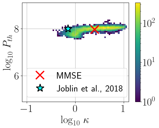
Among other things, the code plots multiple pairplot histograms:

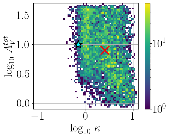
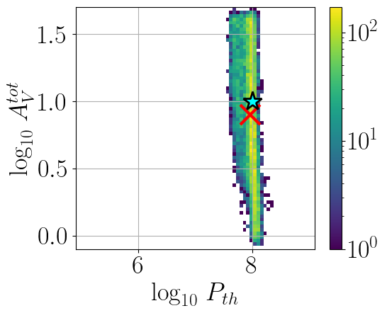
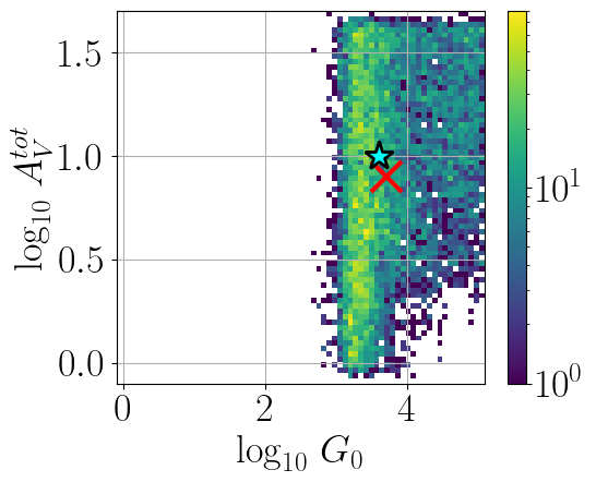
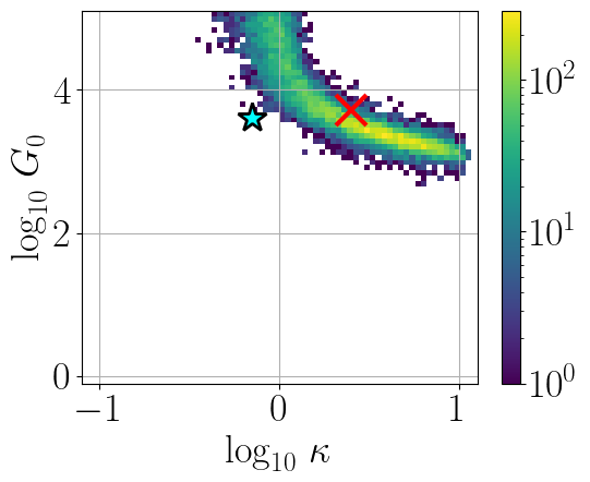
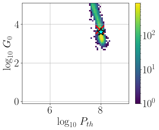
and compares the reproduced observations with the considered observation model (see also the Bayesian p-value):

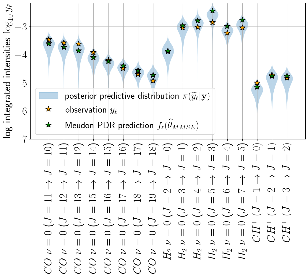
Both the histograms and line predictions are compatible with those found in Joblin et al. [2018].