Sensor localization problem

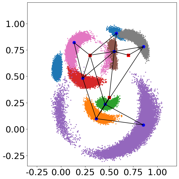
This example shows how the beetroots package can be used to perform inversion on a slightly more complicated case: the sensor localization problem, introduced in Ihler et al. [2005]. This second example appears in Section IV.B of Palud et al. [2023]. The goal is to infer the position of sensors from a set of distance between sensors. The figure below shows the graph of observations with the sensor true positions.

The positions and observed distances are is indicated in the examples/gaussian_mixture/data/sensor_localization_rescaled.csv and observation.csv files, respectively.

Python Simulation preparation

Here are the classes that are necessary to sample from this distribution. The green classes indicate the already implemented classes, and the red classes indicate the classes to implement.

Overall, as

the SmoothIndicatorPrior class, encoding validity intervals
the Posterior class

are already implemented in the base beetroots package, one only needs to implement three classes:

a dedicated ForwardMap class to compute distances between sensors. Can be found in examples/sensor_loc/sensor_loc_forward.
a dedicated Likelihood class to encode the data-fidelity term. Can be found in examples/sensor_loc/sensor_loc_likelihood.
a dedicated Simulation class to set up the observation and posterior. examples/sensor_loc/sensor_loc_simu.

YAML file

input_params_pmtm0p1.py

simu_init:
simu_name: "sensor_loc_pmtm0p1"
max_workers: 10
#
filename_obs: "observation.csv"
#
# prior indicator
prior_indicator:
indicator_margin_scale: 1.0e-2
lower_bounds_lin:
    - -0.35
    - -0.35
upper_bounds_lin:
    - +1.2
    - +1.2
#
likelihood:
R: 0.3
sigma_a: 0.02
#
# sampling params
sampling_params:
mcmc:
    initial_step_size:  3.0e-3
    extreme_grad: 1.0e-5
    history_weight: 0.99
    selection_probas: [0.1, 0.9] # (p_mtm, p_pmala)
    k_mtm: 1_000
    is_stochastic: true
    compute_correction_term: false
#
# run params
run_params:
mcmc:
    N_MCMC: 1
    T_MC: 30_000
    T_BI: 5_000
    plot_1D_chains: true
    plot_2D_chains: true
    plot_ESS: true
    freq_save: 1
    # list_CI: [68, 90, 95, 99]

Sampling

To run the sampling from beetroot’s root folder and save outputs there:

python examples/sensor_loc/sensor_loc_simu.py input_params_pmtm0p9.yaml examples/sensor_loc/data .

where

examples/sensor_loc/sensor_loc_simu.py is the python file to be run
input_params_pmtm0p9.yaml is the yaml file containing the parameters defining the run to be executed
examples/sensor_loc/data : path to the folder containing the yaml input file and the observation data
. : path to the output folder to be created, where the run results are to be saved

To run the sampling from the examples/sensor_loc folder and save outputs there:

cd examples/sensor_loc
python sensor_loc_simu.py input_params_pmtm0p9.yaml ./data .

This run will use a selection probability of 90% for the MTM kernel. To use a 10% selection probability, run

python sensor_loc_simu.py input_params_pmtm0p1.yaml ./data .

The images will be in outputs/sensor_loc_[yyyy]-[mm]-[dd]_[hh]/img. The ESS and MSE values will be in outputs/sensor_loc_[yyyy]-[mm]-[dd]_[hh]/data/output.

Output:

>>> python examples/sensor_loc/sensor_loc_simu.py input_params_pmtm0p9.yaml
starting sampling
starting from a random point
100%|██████████████████████████████████████████████████| 3000/3000 [02:39<00:00, 18.76it/s]
sampling done
N = 8, L (fit) = 11, D_sampling = 2, D = 2
starting clppd plots
starting plot of accepted frequencies
plots of accepted frequencies done
starting plot of log proba accept
plots of log proba accept done
starting plot of objective function
plot of objective function done
100%|███████████████████████████████████████████████████████| 8/8 [00:16<00:00,  2.08s/it]
starting Bayesian p-value plots
Bayesian p-value plots plots done
starting plot proportion of well reconstructed pixels
plot proportion of well reconstructed pixels done
Simulation and analysis finished. Total duration : 00:03:13 s

Sampling results: 2D histograms of the marginal distributions

See Sensor localization: appendix for more details on the construction of the problem.

Identifying incompatible observations

The csv file observation_false.csv contains a distance that was multiplied by 10 to make the set of observations incompatible. When running inference and looking at the marginal distribution, this incompatibility does not appear clearly.

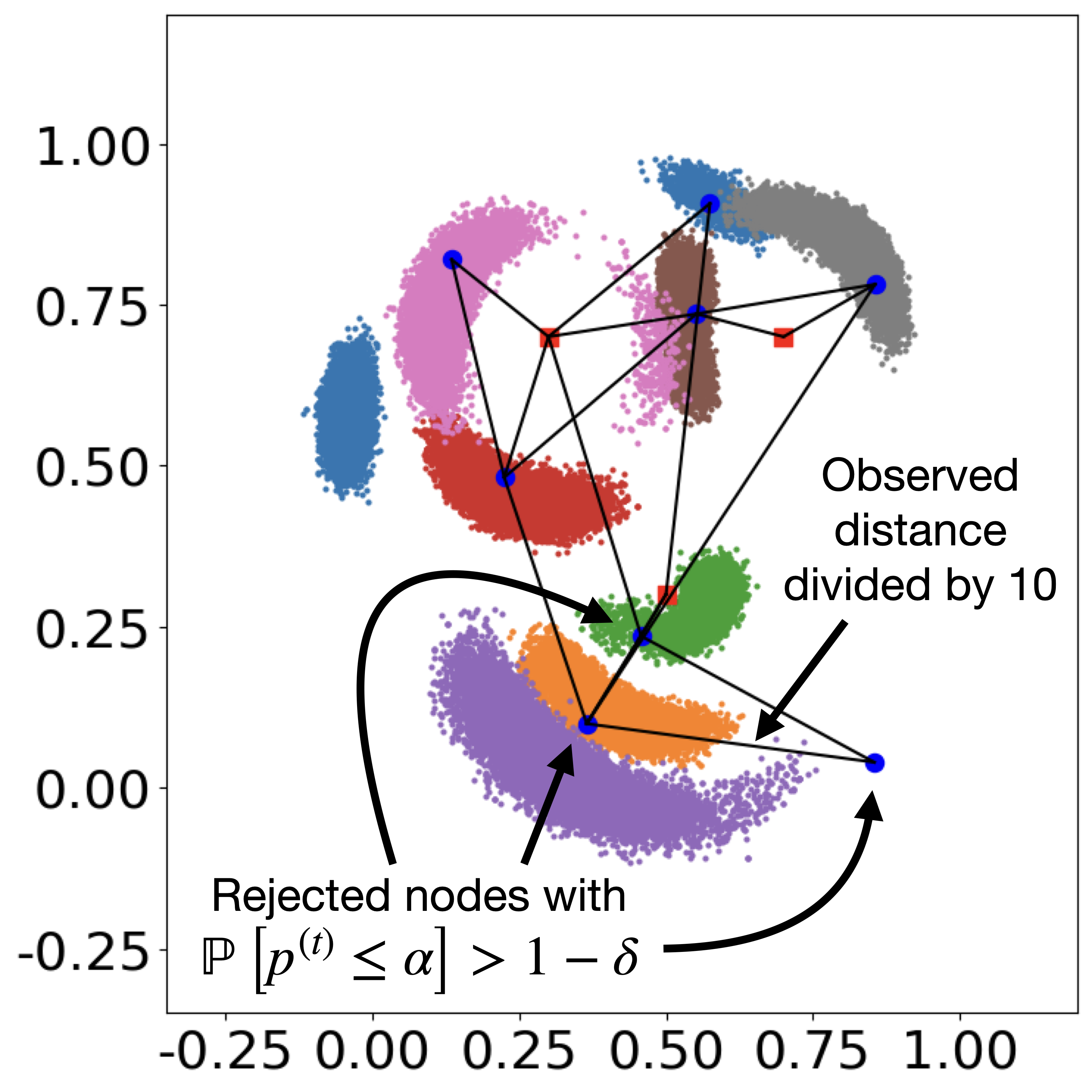
Computing the Bayesian p-value using the method from Palud et al. [2023] permits to identify this incompatibility.

By running

python examples/sensor_loc/sensor_loc_simu.py input_params_pmtm0p9_false.yaml

one can identify the problematic observation. Indeed, the data/output/mcmc/pvalues_analysis.csv file identifies the three sensors that are affected by the alteration. For these three sensors, the reproduced distances are incompatible with the actual observation.

p-value analysis
	n	pval_estim	decision_estim_seed	proba_reject	decision_pval_bayes
0	0	0.639839999999997	1	0.0	1
1	1	7.999999999999923e-05	-1	0.9999971773879514	-1
2	2	3.999999999999932e-05	-1	0.9999999999999689	-1
3	3	0.601720000000003	1	5.112975923355667e-159	1
4	4	0.0	-1	0.9999980518871909	-1
5	5	0.6692000000000052	1	0.0	1
6	6	0.6404000000000029	1	1.1472907567686228e-206	1
7	7	0.6872000000000037	1	0.0	1

In this column:

the seed identifies a run (here only one)
n identifies the sensor
pval_estim provides the Monte Carlo estimator of the p-value
decision_estim_seed corresponds to the decision associated to the estimated p-value, i.e., rejection when \(p \leq \alpha\), with \(\alpha = 0.05\) is a confidence level
proba_reject is the probability that \(p \leq \alpha\) when accounting for uncertainties on the p-value due to the Monte Carlo estimation
decision_pval_bayes corresponds to the decision associated to the rejection probability.

Note

In this table, for the “decision” columns:

“-1” means “reject”, in which case an incompatibility is identified
“0” means “undecided”, in which case the uncertainty on the p-value is too high to take a decision with high confidence
“1” means “no reject”