How to visualize maps
[1]:
import pandas as pd
import numpy as np
import matplotlib.pyplot as plt

from IPython import display

from beetroots.inversion.plots.map_shaper import MapShaper
from beetroots.inversion.plots.plots_2d_setup import Plots2DSetup
from beetroots.inversion.plots.plots_estimator import PlotsEstimator
[2]:
small_size = 16
medium_size = 20
bigger_size = 24

plt.rc("font", size=small_size)  # controls default text sizes
plt.rc("axes", titlesize=small_size)  # fontsize of the axes title
plt.rc("axes", labelsize=medium_size)  # fontsize of the x and y labels
plt.rc("xtick", labelsize=small_size)  # fontsize of the tick labels
plt.rc("ytick", labelsize=small_size)  # fontsize of the tick labels
plt.rc("legend", fontsize=small_size)  # legend fontsize
plt.rc("figure", titlesize=bigger_size)  # fontsize of the figure title
Structure of input files
[3]:
path_data_err = "../data/carina/carina_fts_lines_err_v4_full.pkl"
path_data_int = "../data/carina/carina_fts_lines_int_v4_full.pkl"

df_int = pd.read_pickle(path_data_int)
df_err = pd.read_pickle(path_data_err)

df_int["idx"] = np.arange(len(df_int))
df_err["idx"] = np.arange(len(df_int))
[4]:
df_int.head()
[4]:
| co_v0_j4__v0_j3 | co_v0_j5__v0_j4 | co_v0_j6__v0_j5 | co_v0_j7__v0_j6 | co_v0_j8__v0_j7 | co_v0_j9__v0_j8 | co_v0_j10__v0_j9 | co_v0_j11__v0_j10 | co_v0_j12__v0_j11 | co_v0_j13__v0_j12 | ... | 13c_o_j7__j6 | 13c_o_j8__j7 | 13c_o_j9__j8 | 13c_o_j10__j9 | 13c_o_j11__j10 | 13c_o_j12__j11 | 13c_o_j13__j12 | c_el3p_j1__el3p_j0 | c_el3p_j2__el3p_j1 | idx | ||
|---|---|---|---|---|---|---|---|---|---|---|---|---|---|---|---|---|---|---|---|---|---|---|
| X | Y | |||||||||||||||||||||
| 2 | 9 | 0.000004 | 0.000007 | 0.000011 | 0.000012 | 0.000014 | 0.000011 | 0.000010 | 0.000007 | 0.000004 | 0.000002 | ... | 0.000002 | 0.000001 | 0.000001 | 0.000001 | 1.063700e-06 | 7.964500e-07 | 6.769200e-07 | 0.000001 | 0.000003 | 0 |
| 10 | 0.000004 | 0.000008 | 0.000011 | 0.000012 | 0.000013 | 0.000012 | 0.000010 | 0.000007 | 0.000003 | 0.000002 | ... | 0.000002 | 0.000001 | 0.000001 | 0.000001 | 9.616100e-07 | 8.127100e-07 | 6.397400e-07 | 0.000002 | 0.000004 | 1 | |
| 3 | 7 | 0.000003 | 0.000005 | 0.000008 | 0.000009 | 0.000011 | 0.000012 | 0.000011 | 0.000008 | 0.000005 | 0.000003 | ... | 0.000001 | 0.000001 | 0.000001 | 0.000001 | 4.224100e-07 | 4.775000e-07 | 4.198300e-07 | 0.000001 | 0.000003 | 2 |
| 8 | 0.000006 | 0.000007 | 0.000011 | 0.000013 | 0.000015 | 0.000014 | 0.000012 | 0.000008 | 0.000005 | 0.000003 | ... | 0.000002 | 0.000001 | 0.000001 | 0.000001 | 5.350700e-07 | 5.279300e-07 | 4.875700e-07 | 0.000001 | 0.000003 | 3 | |
| 9 | 0.000006 | 0.000009 | 0.000013 | 0.000014 | 0.000016 | 0.000014 | 0.000012 | 0.000008 | 0.000004 | 0.000003 | ... | 0.000002 | 0.000001 | 0.000001 | 0.000001 | 6.908500e-07 | 6.093400e-07 | 6.810400e-07 | 0.000002 | 0.000004 | 4 |
5 rows × 22 columns
The index of the two files containing the integrated intensities and the error standard deviations is (X, Y), i.e., horizontal and vertical position.
This index permits to describe for non-recangular images. Such images are typically difficult to handle with matplotlib as they require to use a wide rectangular array with NaNs.
We built three classes to better handle such non-rectangular maps:
MapShaperpermits to convert a vector that contains only relevant values to a plotable image.Plots2DSetupcontains multiple methods to plot figures relative to the setup of an inversion.PlotsEstimatorpermits to plot estimated physical conditions.
MapShaper : how to convert a vector to a map
[5]:
y = df_int.loc[:, "co_v0_j4__v0_j3"].values
y.shape
[5]:
(176,)
[6]:
map_shaper = MapShaper(df_int)
y_shaped = map_shaper.from_vector_to_map(y)

y_shaped
[6]:
array([[       nan,        nan,        nan,        nan, 9.3880e-07,
               nan,        nan,        nan,        nan,        nan,
               nan,        nan,        nan,        nan,        nan,
               nan,        nan,        nan,        nan,        nan,
               nan,        nan,        nan],
       [       nan,        nan, 2.8629e-06,        nan, 1.6018e-06,
        1.6818e-06, 7.1836e-07,        nan,        nan,        nan,
               nan,        nan,        nan,        nan,        nan,
               nan,        nan,        nan,        nan,        nan,
               nan,        nan,        nan],
       [       nan, 2.9443e-06, 2.8852e-06, 3.0009e-06, 2.5902e-06,
        1.5138e-06, 8.2986e-07, 1.0882e-06,        nan,        nan,
               nan,        nan,        nan,        nan,        nan,
               nan,        nan,        nan,        nan,        nan,
               nan,        nan,        nan],
       [       nan, 6.0927e-06, 5.6067e-06, 3.8729e-06, 2.5838e-06,
        1.3390e-06, 9.2523e-07, 8.3533e-07,        nan,        nan,
               nan,        nan,        nan,        nan,        nan,
               nan,        nan,        nan,        nan,        nan,
               nan,        nan,        nan],
       [4.0794e-06, 6.3580e-06, 5.3340e-06, 4.0676e-06, 1.7101e-06,
        1.5886e-06, 1.4857e-06, 9.8363e-07, 1.1935e-06, 2.2821e-06,
        2.5388e-06,        nan,        nan,        nan,        nan,
               nan,        nan,        nan,        nan,        nan,
               nan,        nan,        nan],
       [4.1535e-06, 6.8713e-06, 5.3752e-06, 3.1585e-06, 2.0418e-06,
        2.2476e-06, 1.6425e-06, 1.4960e-06, 1.7269e-06, 3.0545e-06,
        3.4925e-06,        nan, 5.9910e-06,        nan,        nan,
               nan,        nan,        nan,        nan,        nan,
               nan,        nan,        nan],
       [       nan, 5.0684e-06, 4.0796e-06, 4.0307e-06, 3.1467e-06,
        3.2164e-06, 2.9036e-06, 2.2017e-06, 3.2037e-06, 5.2519e-06,
        5.4572e-06, 5.9301e-06, 5.0309e-06, 4.5744e-06,        nan,
               nan,        nan,        nan,        nan,        nan,
               nan,        nan,        nan],
       [       nan,        nan, 3.1179e-06, 2.6436e-06, 3.2860e-06,
        3.5291e-06, 3.9545e-06, 3.4073e-06, 4.2027e-06, 5.6134e-06,
        5.8476e-06, 5.9051e-06, 3.7806e-06, 3.7117e-06, 4.3941e-06,
               nan,        nan,        nan,        nan,        nan,
               nan,        nan,        nan],
       [       nan,        nan,        nan,        nan, 3.8429e-06,
        4.6323e-06, 4.2567e-06, 3.7124e-06, 4.0153e-06, 5.3059e-06,
        5.1337e-06, 4.0326e-06, 4.2778e-06, 4.6504e-06, 3.5612e-06,
               nan, 5.4571e-06,        nan,        nan,        nan,
               nan,        nan,        nan],
       [       nan,        nan,        nan,        nan,        nan,
               nan, 3.7285e-06, 3.3062e-06, 3.4754e-06, 3.5539e-06,
        3.4852e-06, 4.2932e-06, 5.2816e-06, 5.2725e-06, 4.9149e-06,
        5.0087e-06, 5.0891e-06, 4.8088e-06,        nan,        nan,
               nan,        nan,        nan],
       [       nan,        nan,        nan,        nan,        nan,
               nan, 3.7676e-06, 3.0847e-06, 2.5616e-06, 2.8786e-06,
        3.1190e-06, 4.5977e-06, 5.3041e-06, 5.3624e-06, 5.1987e-06,
        5.2091e-06, 5.2683e-06, 7.0245e-06,        nan,        nan,
               nan,        nan,        nan],
       [       nan,        nan,        nan,        nan,        nan,
               nan,        nan,        nan,        nan, 2.5504e-06,
        2.7641e-06, 3.5819e-06, 5.1698e-06, 5.0090e-06, 5.3889e-06,
        5.7985e-06, 6.6326e-06, 9.0326e-06, 1.5794e-05, 2.0978e-05,
               nan,        nan,        nan],
       [       nan,        nan,        nan,        nan,        nan,
               nan,        nan,        nan,        nan, 1.5634e-06,
        2.4211e-06, 3.1557e-06, 3.2835e-06, 3.6685e-06, 4.5759e-06,
        6.4911e-06, 1.0774e-05, 1.4629e-05, 1.6757e-05, 2.1450e-05,
               nan,        nan,        nan],
       [       nan,        nan,        nan,        nan,        nan,
               nan,        nan,        nan,        nan,        nan,
        2.4599e-06, 2.5915e-06, 2.0976e-06, 3.2115e-06, 3.9609e-06,
        6.6847e-06, 1.0575e-05, 1.6988e-05, 2.5206e-05, 2.5327e-05,
               nan, 2.2669e-05,        nan],
       [       nan,        nan,        nan,        nan,        nan,
               nan,        nan,        nan,        nan,        nan,
               nan,        nan, 1.9075e-06, 3.0966e-06, 2.8063e-06,
        6.5508e-06, 8.9596e-06, 1.8592e-05, 2.4915e-05, 2.4467e-05,
        2.3575e-05, 2.2669e-05, 2.3402e-05],
       [       nan,        nan,        nan,        nan,        nan,
               nan,        nan,        nan,        nan,        nan,
               nan,        nan,        nan, 2.9698e-06,        nan,
        5.6569e-06, 8.4912e-06, 2.0885e-05, 2.4379e-05, 2.4400e-05,
        2.2950e-05, 2.0715e-05, 2.5673e-05],
       [       nan,        nan,        nan,        nan,        nan,
               nan,        nan,        nan,        nan,        nan,
               nan,        nan,        nan,        nan,        nan,
        5.8810e-06, 1.6289e-05, 1.8142e-05, 2.2382e-05, 2.3170e-05,
        2.3210e-05, 2.1786e-05, 2.6933e-05],
       [       nan,        nan,        nan,        nan,        nan,
               nan,        nan,        nan,        nan,        nan,
               nan,        nan,        nan,        nan,        nan,
        5.5943e-06, 1.2833e-05, 1.5005e-05, 2.1013e-05, 2.1763e-05,
        2.4136e-05, 2.5732e-05, 2.6437e-05],
       [       nan,        nan,        nan,        nan,        nan,
               nan,        nan,        nan,        nan,        nan,
               nan,        nan,        nan,        nan,        nan,
               nan,        nan,        nan, 1.5583e-05, 1.4004e-05,
        1.5987e-05,        nan,        nan]])
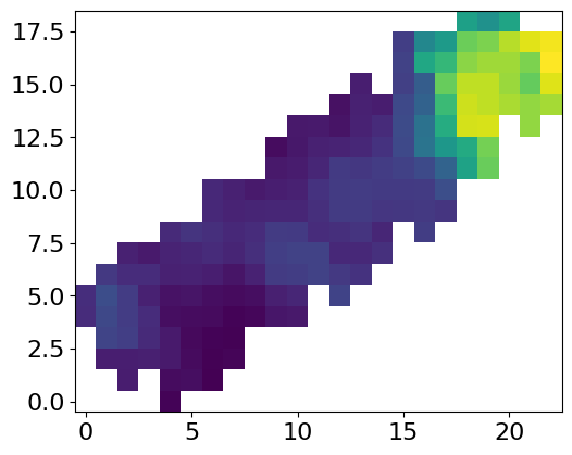
[7]:
plt.imshow(y_shaped, origin="lower")
plt.show()
Plot2DSetup : Already implemented methods to plot observations
[8]:
path_img = "img/create_input_files"
N = len(df_int)

setup_plotter = Plots2DSetup(path_img, map_shaper, N)
[9]:
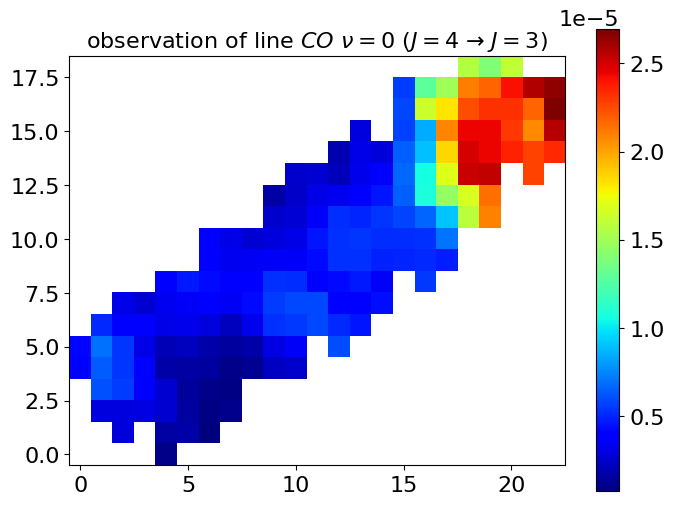
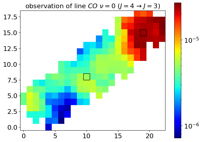
# choose the lines to plot
list_lines = ["co_v0_j4__v0_j3", "co_v0_j5__v0_j4"]

setup_plotter.plot_observations(
    y=df_int.loc[:, list_lines].values, list_lines=list_lines, folder_path=path_img
)
[10]:
display.Image(f"{path_img}/observation_line_0_co_v0_j4__v0_j3_linscale.PNG")
[10]:
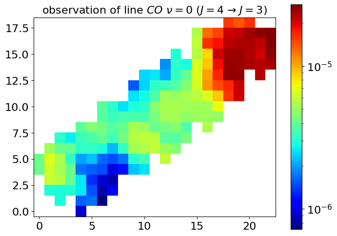
[11]:
display.Image(f"{path_img}/observation_line_0_co_v0_j4__v0_j3.PNG")
[11]:
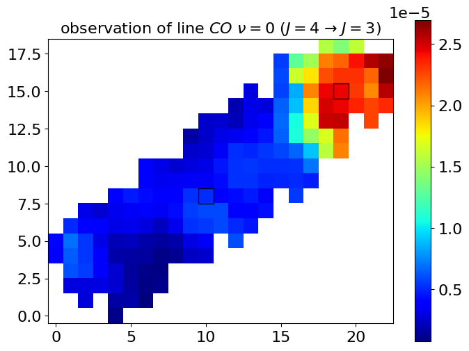
It is also possible to highlight some pixels. To do so, simply provide a dictionary of (index, name) pairs:
[12]:
setup_plotter = Plots2DSetup(
    path_img, map_shaper, N, pixels_of_interest={158: "Car-I", 76: "Car-I/II"}
)

setup_plotter.plot_observations(
    y=df_int.loc[:, list_lines].values, list_lines=list_lines, folder_path=path_img
)
[13]:
display.Image(f"{path_img}/observation_line_0_co_v0_j4__v0_j3_linscale.PNG")
[13]:
[14]:
display.Image(f"{path_img}/observation_line_0_co_v0_j4__v0_j3.PNG")
[14]:
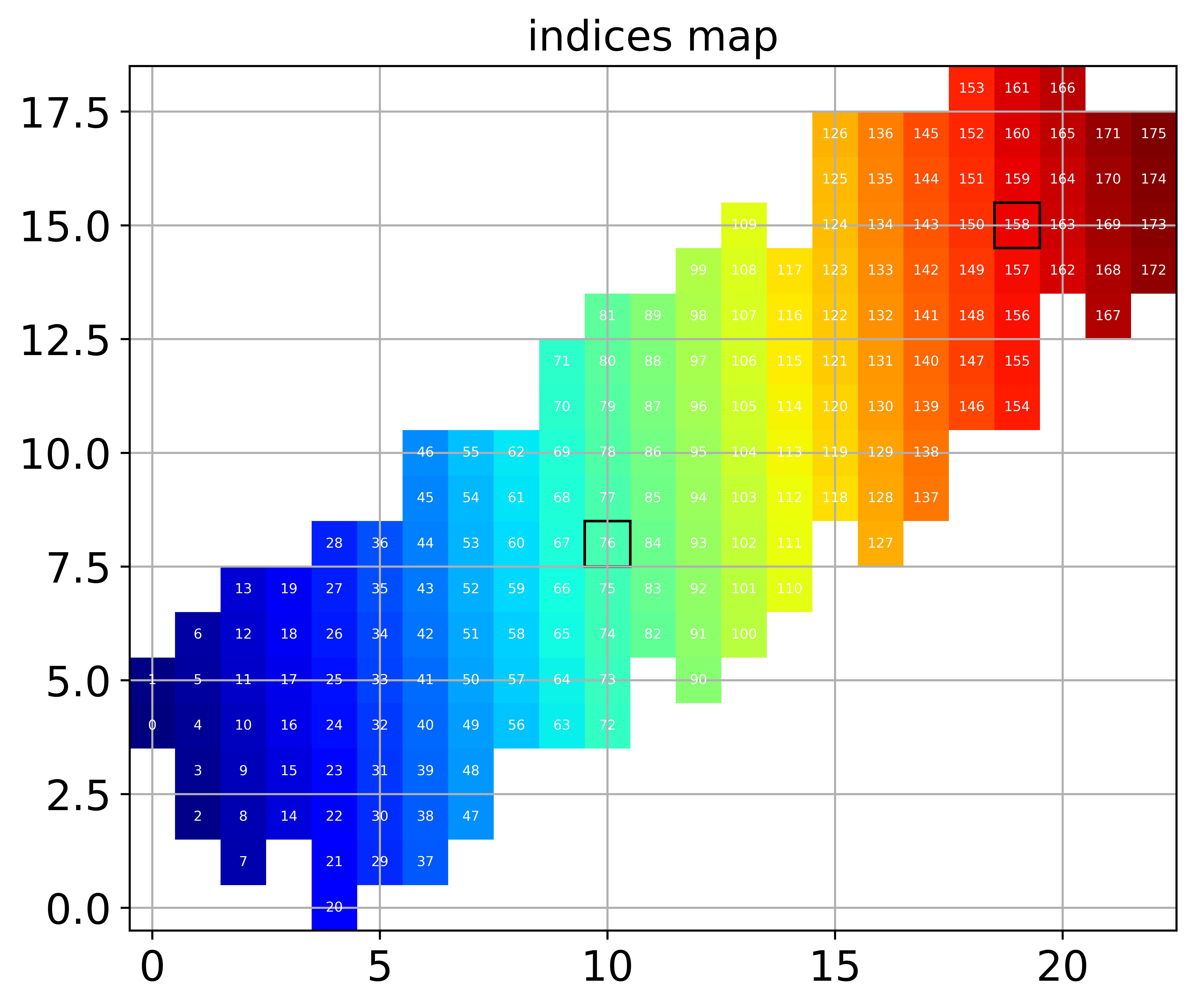
To check the indices to highlight the pixel you are interested in, plot the map of indices :
[15]:
setup_plotter.plot_indices_map()

display.Image(f"{path_img}/indices_map.PNG")
[15]:
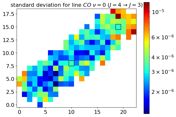
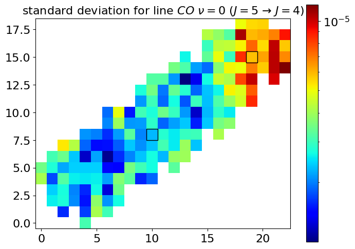
You may also want to plot the additive noise standard deviation :
[16]:
setup_plotter.plot_sigma_a(
    sigma_a=df_err.loc[:, list_lines].values,
    list_lines=list_lines,
    folder_path=path_img,
)
[17]:
display.Image(f"{path_img}/add_err_std_line_0_co_v0_j4__v0_j3.PNG")
[17]:
[18]:
display.Image(f"{path_img}/add_err_std_line_1_co_v0_j5__v0_j4.PNG")
[18]:
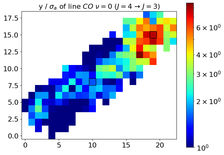
Finally, to assess the Signal to noise ratio (SNR):
[19]:
setup_plotter.plot_snr_add(
    y=df_int.loc[:, list_lines].values,
    sigma_a=df_err.loc[:, list_lines].values,
    list_lines=list_lines,
    folder_path=path_img,
)
[20]:
display.Image(f"{path_img}/snr_line_0_co_v0_j4__v0_j3.PNG")
[20]:
[21]:
display.Image(f"{path_img}/snr_line_1_co_v0_j5__v0_j4.PNG")
[21]:
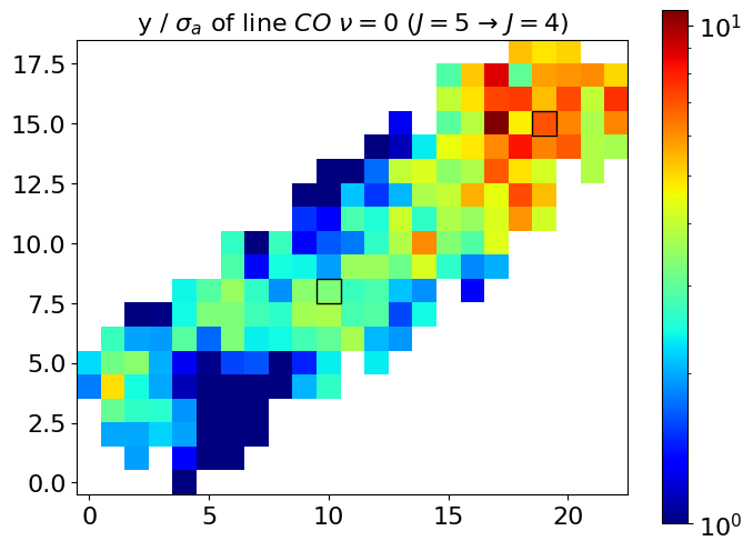
In the case of the Carina Nebula, these figures show the variation of SNR, with a bright and high SNR region at the top of the map, and a dark and low SNR region in the bottom.
PlotEstimators : Already implemented methods to plot inference results
[22]:
# load estimations from Wu et al. (2018)
df_wu2018 = pd.read_pickle("../data/carina/values_wu_et_al_2018.pkl")

df_wu2018.head()
[22]:
| kappa | P | radm | Avmax | alpha | ||
|---|---|---|---|---|---|---|
| X | Y | |||||
| 2 | 9 | 1.0 | 6.851674e+07 | 10010.458030 | 10.0 | 0.0 |
| 10 | 1.0 | 7.702090e+07 | 12538.628139 | 10.0 | 0.0 | |
| 3 | 7 | 1.0 | 8.526743e+07 | 16992.703471 | 10.0 | 0.0 |
| 8 | 1.0 | 8.526743e+07 | 13164.397808 | 10.0 | 0.0 | |
| 9 | 1.0 | 8.292417e+07 | 12968.686817 | 10.0 | 0.0 |
One can see that the index matches the index of the observations.
[23]:
estimator_plotter = PlotsEstimator(
    map_shaper,
    list_names=[r"$\kappa$", r"$P_{th}$", r"$G_0$", r"A_V^{tot}$", r"$\alpha$"],
    lower_bounds_lin=np.array([0.1, 1e5, 1.0, 1.0, 0.0]),
    upper_bounds_lin=np.array([10.0, 1e9, 1e5, 40.0, 0.0]),
    list_idx_sampling=list(range(5)),
)
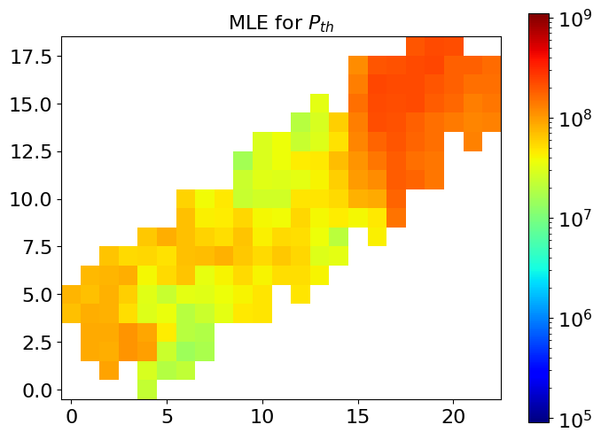
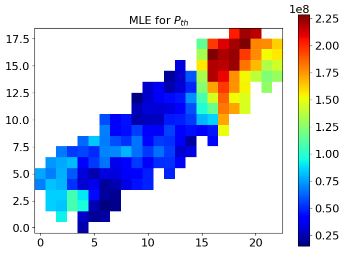
[24]:
estimator_plotter.plot_estimator(
    Theta_estimated=df_wu2018.values, estimator_name="MLE", folder_path=path_img
)
[25]:
display.Image(f"{path_img}/MLE_1.PNG")
[25]:
[26]:
display.Image(f"{path_img}/MLE_linscale_1.PNG")
[26]:
This class also contains other methods, for instance that can be used to illustrate credibility intervals.